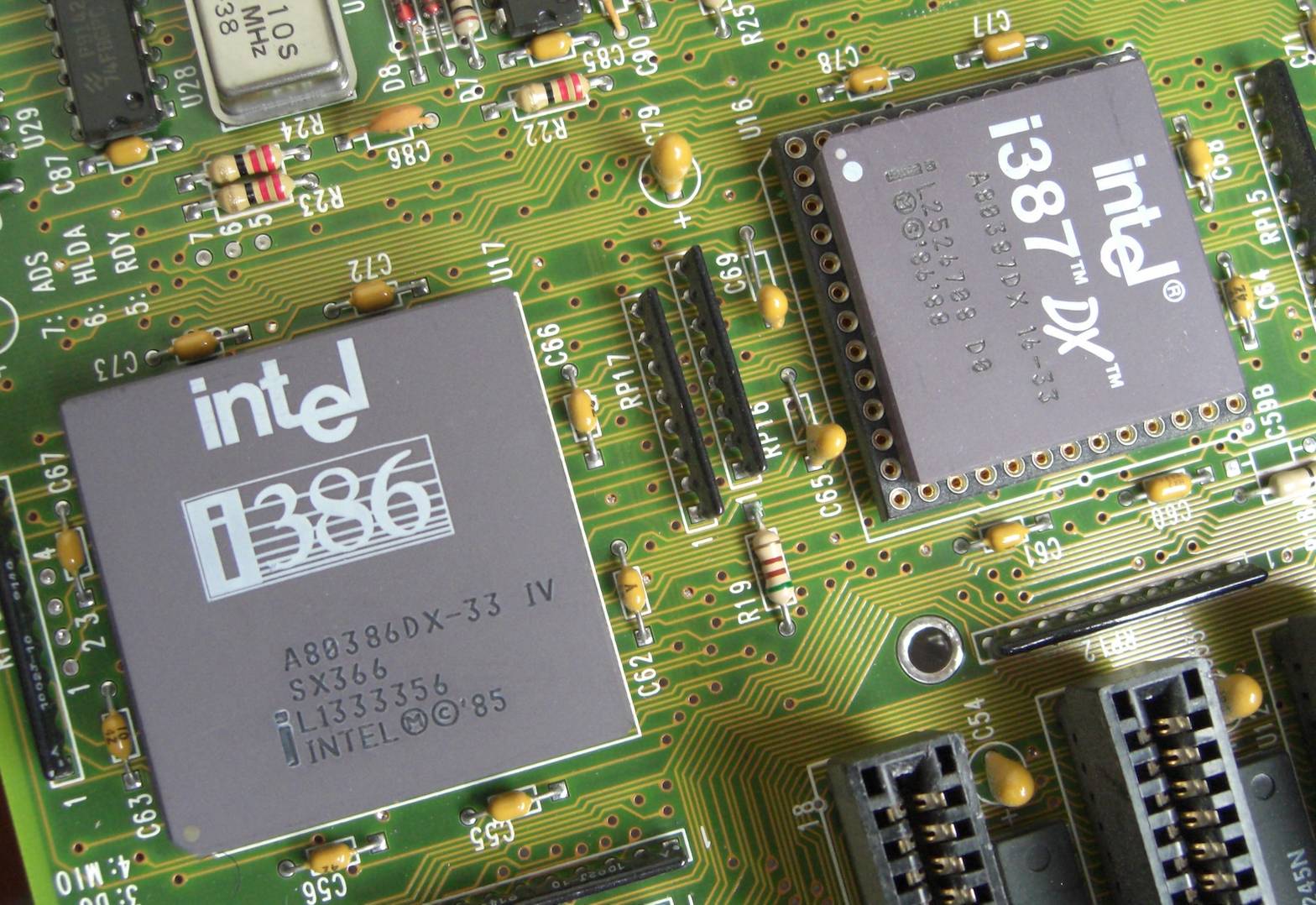
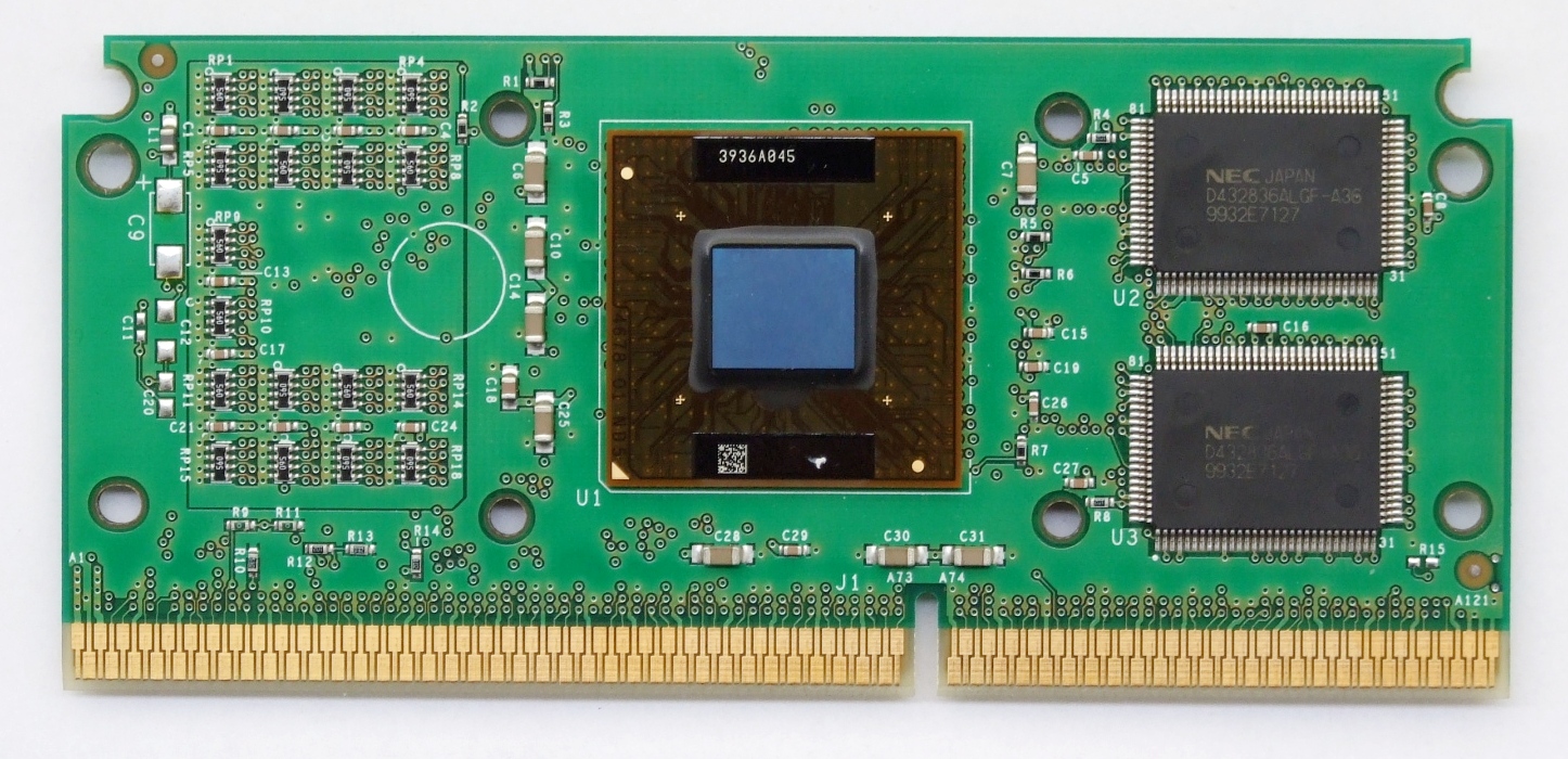
Thinking back about the past is a side effect of getting older. So when I recently configured a new workstation, I couldn’t help thinking back about my first PC. I had bought it in 1993, a 386DX-40 with 4 MB of RAM and a 170 MB hard disk drive – a major leap forward compared to the Commodore 64 that I had at my disposal before that, unless I got on my bike for a trip to the neighbouring village and access to my uncle’s old 286. Nevertheless, despite a meantime upgrade to a 486DX-50, this computer was very much obsolete six years later. That’s why I replaced it in 1999 with a Pentium III 450 with 128 MB of RAM and a 10 GB hard disk. This computer provided my computing needs during my time at the university. On the operating system side, I went from MS-DOS 6.22 and Windows 3.11 to Windows 98 SE and SuSE Linux.
What a difference compared to modern days – my old workstation, now also more than six years old, is still doing its job faithfully even after processing many terabytes of point clouds. It is suitable for Windows 11 and it’s mostly the video card that could use an upgrade. Does this mean that there have really been only minor advances in recent years when it comes to computing power?
An proper assessment requires measuring performance and placing it in the historical contact. Measuring is done with benchmarks – popular choices are Cinebench and Geekbench. But these don’t run on old hardware, which makes a comparison of many generations of computers impossible.
In the domain of supercomputers and scientific computations, the most important performance measure is how fast numerical computations with floating point numbers can be performed. This computin speed is expressed in FLOPS, which stands for floating point operations per second. For supercomputers, this is measured with the LINPACK benchmark that constructs and solves systems of linear equations – something that geodesists are familiar with as parameter estimation with least squares. LINPACK measures the speed when processing 64-bit numbers, known as double precision. 32-bit numbers are single precision.
The fun part is that a lot of historical FLOPS measurements and LINPACK results are available for a comparison of systems throughout several decades. For PCs, you realistically can’t go back beyond the 486 CPU, as it was the first x86 CPU with a built-in floating point unit (FPU). The 386 and earlier CPUs emulated these in software, which was very slow – unless you bought an external math coprocessor, which in case of the 386 was called the 387.
So let’s first take a look at supercomputers to be able to go back in time even further. The first computers, such as the Zuse Z3 and ENIAC, were developed for scientific computations. The electro-mechanic Z3 needed almost a second for adding two numbers. ENIAC was already much faster with several thousand calculations per second. But the distinction between supercomputers and “normal” computers wasn’t really made until the 1960s, when the general use of computers really took off. And with “normal” computers, we are of course talking about room-filling mainframes like IBM’s System/360, the best-selling computer family in that time.
In 1964, Control Data Corporation launched its CDC 6600, which is usually considered to be the first true supercomputers. It achieved 3 MFLOPS, i.e. three million calculations per second..
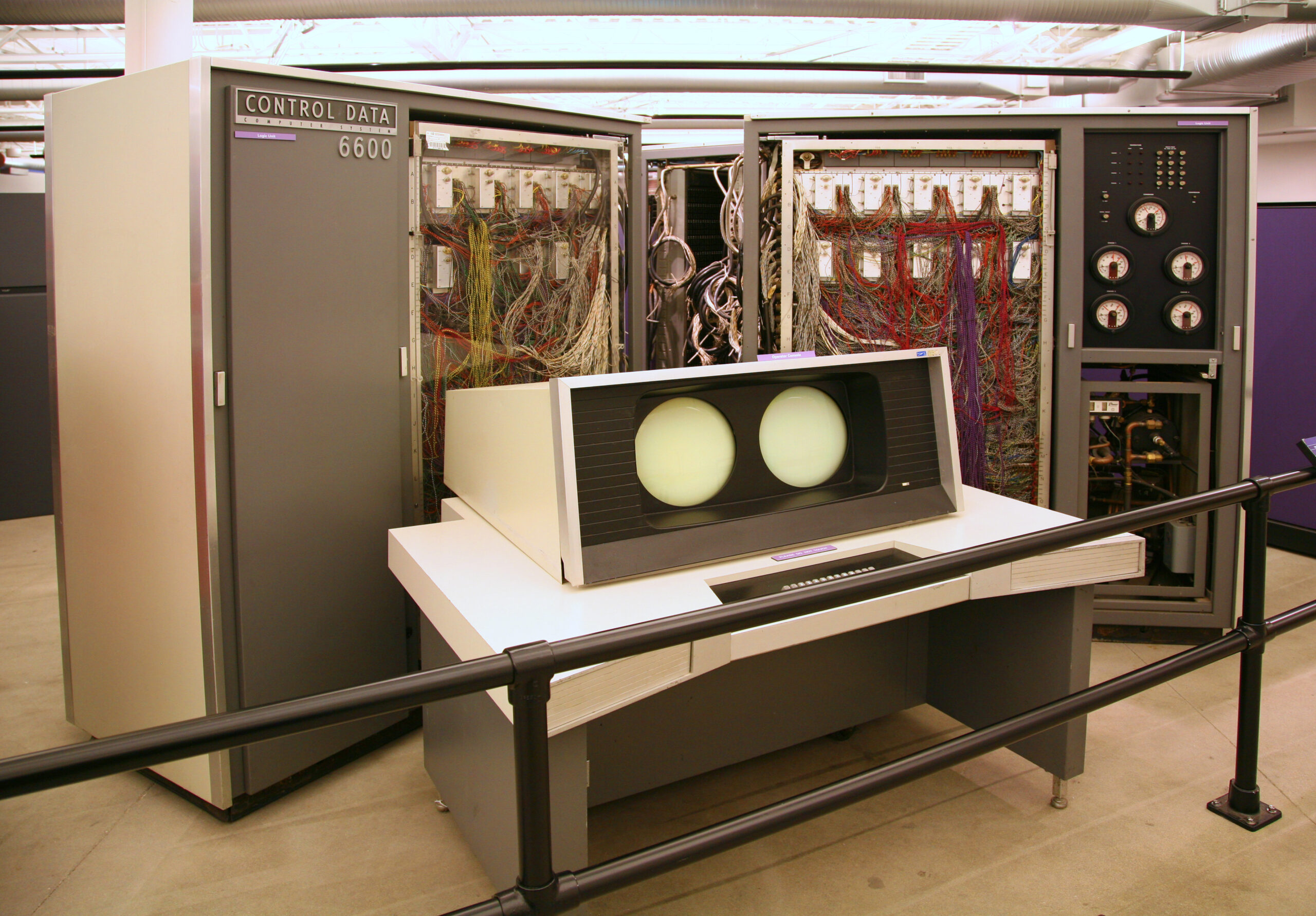
The CDC 6600 had been designed by a certain Seymour Cray. This name might ring a bell with some of the readers. In 1972, he started his own company: Cray Research. Ever since, Cray is almost synonymous with supercomputers.
The Cray X-MP was a successful model and the fastest computer in the world from 1983 to 1985, at 800 MFLOPS – almost 300 times the speed of the CDC 6600. This despite being a relatively compact system that looked more like a piece of design furniture. The successor Y-MP broke through the GFLOPS barrier with more than 2 billion computations per second. Typical characteristics of the Crays of that era are the use of vector processors (that operate not on single numbers, but several at once) and liquid cooling.

NEC in Japan also used vector processors in its SX range. But a new trend arrived in the 90s. Instead of using custom vector processors, supercomputers increasingly used very large numbers of much cheaper “standard” CPUs. Cray followed suit with its T3E range that used DEC’s Alpha CPUs. The fastest incarnation of the T3E scored 891 GFLOPS, making it 1000 times faster than the X-MP of 15 years prior. A list of the 500 fastest computers in the world is published twice a year since 1993 – the TOP500 list. In June of 2000, this fastest version of the T3E was ranked #7.
My first real contact with supercomputers was during a visit to the Höchstleistungsrechenzentrum Stuttgart (HLRS) in 2003 that I had organised for geodesy students. At the time, the HLRS had both a NEC SX-5 and a Cray T3E. The latter was housed at Daimler, who billed by square meter of floor space – which was advantageous with the compact liquid-cooled T3E. The air-cooled systems were located in HLRS’s own halls. Why two systems? Massively parallel systems require other programming techniques than vector systems, which leads to some applications being more suitable to one or the other.
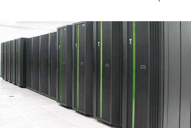
In the meantime, a third architecture had gained popularity: clusters, constructed from normal servers or workstations, but often with a faster network connection. Being made form off-the-shelf components and lacking the fast internal interconnect of “real” supercomputers made these quite a bit cheaper, but once again not suitable for each application.
I wanted to work with supercomputers for my master thesis project. In geodesy, this means gravity field modelling. As a result, I spent five months of 2004 parallelising algorithms for gravity field parameter estimation from satellite observations and testing them on the HLRS systems. HLRS had just ordered a new system from NEC and received an SX-6 installation as temporary solution until the new system was ready, and we were given access and computing time on it. There was a queue, of course, which meant that you would often wait hours or even days until your job ran. We “solved” this by running computations on the TX-7 front-end system, which thanks to 16 Itanium II CPUs wasn’t exactly slow either…
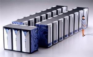
NEC was a big name in those days, as they had delivered the Earth Simulator in 2002. With a speed of 36 TFLOPS, it was five times faster than the number two on the TOP500 list and stayed on top for more than two years. The TFLOPS barrier had already been broken through in 1997, by the massively parallel ASCI Red that was powered by Intel Pentium Pro CPUs.
After graduating from the University of Stuttgart, I started as PhD candidate at the Delft University of Technology. We initially had access to the Dutch national supercomputers TERAS and ASTER. Even better, in 2005 we were granted the funds to buy our own cluster. This system that I had christened CLEOPATRA consisted of 33 nodes (individual computers) connected via Infiniband with a maximum speed in excess of 600 GFLOPS. Five years earlier, this would have been sufficient for a spot in the top 10% of the TOP500 list.
Towards the end of my PhD research, I had out-grown CLEOPATRA, especially with regard to RAM. I applied a filtering technique on which an audience member during a presentation of mine commented “I was told this wasn’t feasible”. It was – if you had enough computing power. In 2009, this was provided by the new national supercomputer Huygens 2, a 60 TFLOPS system – 100 times the speed of our CLEOPATRA.
Now, 15 years later, 60 TFLOPS isn’t impressive any more. The “slowest” system on November 2025’s TOP500 list reaches 2.5 PFLOPS. But we have already arrived in the Exascale era – the fastest computer at the time of writing is El Capitan with 1.7 EFLOPS top speed. It was built by Cray, now a subsidiary of HP. The comparison of modern supercomputers to those of the previous century is slightly unfair, as they now always are networked modular systems that often fill entire halls, and no longer relatively compact monolitihic systems. This means that computing power is not limited by what a single system delivers. but only by money, space, and electrical power supply.

But lets go back to computers for ordinary people. My 486DX-50 probably achieved around 2 MFLOPS, so a bit less than the CDC 6600 of 30 years prior. The Pentium III 450 achieved more than 60 MFLOPS. The speed increase was the result not only of the increase in CPU clock speed, but also of faster calculations due to improvements to the GPU. The 800 MFLOPS of the Cray X-MP were matched by the 3 GHz version of the Pentium 4 that was released in 2002 – in just three and a half years, Intel had gone from 450 MHz to 3 GHz and from 60 to 800 MFLOPS.
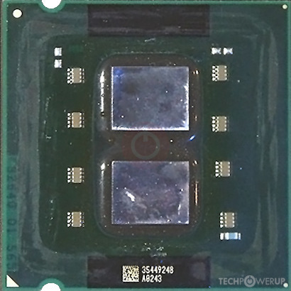
The Pentium 4 wasn’t a very efficient design, but at the end of its lifecycle, it brought two important innovations that are now used in all x86 CPUs: the 64-bit extension to the x86 standard that had been developed by AMD, and the first dual-core processor, with two almost independent processing units on a single CPU. I was the first employee at Delft’s Aerospace Engineering department with a computer powered by this Pentium D under his desk. It provided enough computing power until CLEOPATRA became available.
So far, I’ve always talked about LINPACK results for getting FLOPS as measure of computing speed. I want to give everyone a shot at running a benchmark, but the full LINPACK benchmark might be a bit much for the average computer and too difficult to install. An important part of it is matrix-matrix multiplication. This can be optimised quite well, which means that many computers come close (and by that I mean 50% or better) to their theoretical peak performance. The Pentium D could in theory perform two floating point operations per core per clock cycle, which yields a theoretical peak of 12 GFLOPS at a clock frequency of 3 GHz. I’ve found old benchmark results of mine that stated almost 11 GFLOPS, i.e. around 90% of the theoretical peak. I’m not sure why the LINPACK results that I’ve found for the normal Pentium 4 are so much lower, maybe because the more inefficient solving of the linear equation systems counts here as well? In any case, 11 GFLOPS would have been enough for the 111th spot on the TOP500 list of 10 years earlier.
In the 20 years since then, progress hasn’t stood still. Sure, CPU clock speeds turned out to be limited, and we now have turbo burst speeds of close to 6 GHz, approx. twice that of the Pentium 4 of 20 years ago. But two things have grown considerably: the number of cores if a CPU (an AMD Ryzen 9 9950X has 16 identical cores, an Intel Core Ultra 9 285 even 24 of them of two types, performance and efficiency), and the number of operations performed per clock cycle – now up to 32.
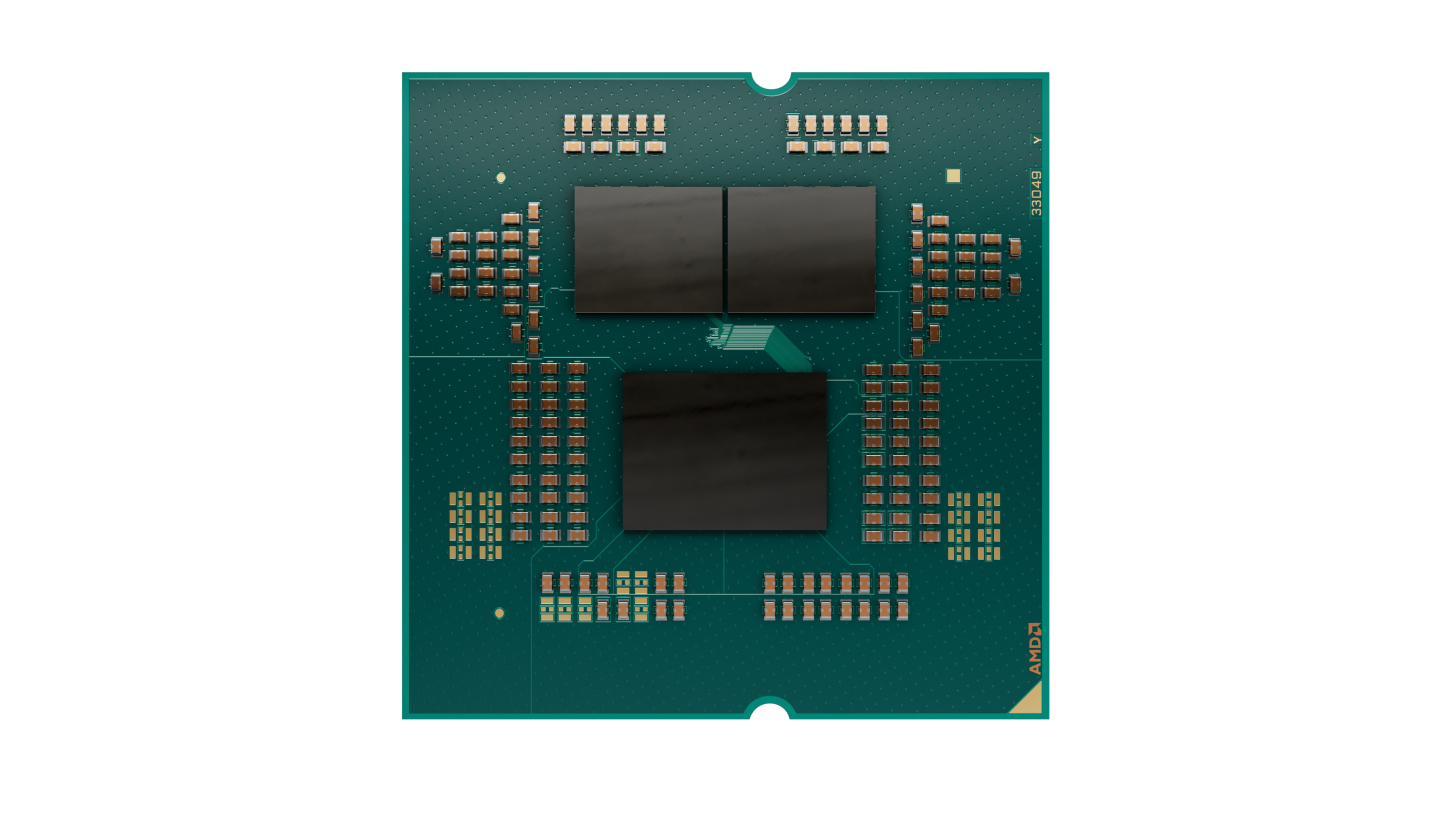
This means that a Ryzen9 9950X has a theoretical peak performance in excess of 2 TFLOPS. I happen to have one under my desk, and I measure 1.4 TFLOPS with a benchmark program written in Python – more than 100 times the speed of the Pentium D of 20 years ago. My old workstation, equipped with an Intel Core i5-9600K, reaches 250 GFLOPS, a little more than a sixth.
But wait a second, doesn’t everyone use GPUs or accelerators derived from them these days? Let’s take a look at the performance of Nvidia’s top model for gaming, the RTX 5090. I measure just 1.5 TFLOPS or 10% more than the CPU – what a disappointment!
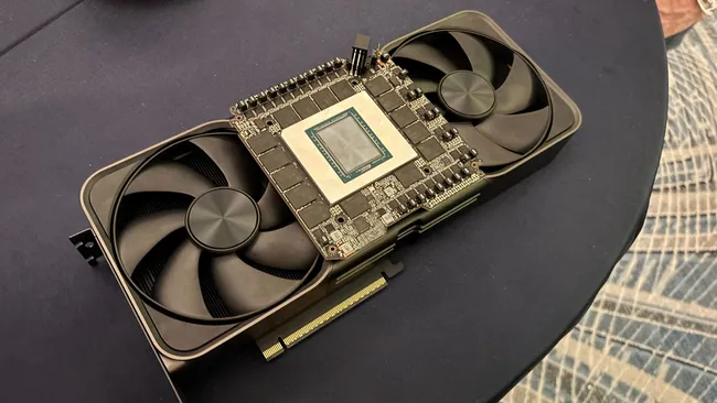
The reason? Nvidia’s consumer GPUs and the derived workstation GPUs are very slow when it comes to 64-bit double-precision calculations. You can also run the benchmark with 32-bit single-precision number. I then get 3.2 TFLOPS for the Ryzen 9 9950X, and (depending on the matrix size) 25 to 30 TFLOPS for the RTX 5090 – 16 times faster than in dual precision. For those requiring full computing power in double precision, you’ll have to shell out much more money for one of the high-end GPUs. The RTX 2070 in my old workstation did already 5 TFLOPS in single precision, so here the progress over 5 years is even less than on the CPU side.
So no, computing power isn’t growing as quickly as it did 25 years ago, when we had tenfold increases in three years. As a result, supercomputers have opened the gap again. Where a Pentium D would have been relatively close to the TOP500 list 10 years earlier, this is no longer the case for the Ryzen 9 9950X – in 2015, you needed 200 TFLOPS to even make the list.
But is this bad? I don’t think so. We’ve arrived at a point where a computer from a couple of years ago is still performing fine for the daily tasks, which often happen in a web browser anyway. The general impression is that it’s mostly the gamers that demand ever more power. As a result, we also see a shift in attention towards computing efficiency instead of computing power only. A laptop that runs an entire day on a single battery charge, just a dream a couple of years ago, is now reality. Even with supercomputers, efficiency is increasingly in the spotlights – there’s now also a GREEN500 list that ranks systems by GFLOPS per watt of consumed energy.
Sources
https://en.wikipedia.org/wiki/Floating_point_operations_per_second
http://www.roylongbottom.org.uk/linpack%20results.htm
Wittwer, T.: An Introduction to Parallel Programming. PDF.
Benchmark code
This code was written by Github Copilot and extended by me with the use of CuPy. You’ll need a suitable Nvidia GPU, the CUDA Toolkit and of course CuPy.
import argparse
import time
from typing import Tuple, Callable, Dict
import numpy as np
import cupy as cp

#!/usr/bin/env python3
"""
Matrix-matrix multiplication benchmark.

Usage examples:
    python bench_matmul.py --sizes 256 512 --repeats 3 --methods numpy python einsum
    python bench_matmul.py --size 1024 --repeats 5
"""

def parse_args():
        p = argparse.ArgumentParser(description="Matrix-matrix multiplication benchmark")
        p.add_argument("--sizes", "-s", nargs="+", type=int, default=[256, 512, 1024, 8192],
                                     help="Square matrix sizes to benchmark (space separated).")
        p.add_argument("--repeats", "-r", type=int, default=3, help="Number of repetitions per test.")
        p.add_argument("--dtype", "-d", choices=["float64", "float32"], default="float64")
        p.add_argument("--seed", type=int, default=42, help="Random seed")
        p.add_argument("--methods", "-m", nargs="+",
                                     choices=["numpy", "einsum", "python", "cupy"],
                                     default=["numpy", "einsum","cupy"],
                                     help="Which implementations to run.")
        return p.parse_args()

def make_matrices(n: int, dtype=np.float64, seed: int = 0) -> Tuple[np.ndarray, np.ndarray]:
        rng = np.random.default_rng(seed + n)
        A = rng.standard_normal((n, n), dtype=dtype)
        B = rng.standard_normal((n, n), dtype=dtype)
        return A, B

def ops_count(n: int) -> int:
        # For square n x n: 2*n^3 floating-point operations (mul + add)
        return 2 * (n ** 3)

def bench(func: Callable[[np.ndarray, np.ndarray], np.ndarray],
                    A: np.ndarray, B: np.ndarray, repeats: int) -> Tuple[float, np.ndarray]:
        # warm up
        C = func(A, B)
        t0 = time.perf_counter()
        for _ in range(repeats):
                C = func(A, B)
        t1 = time.perf_counter()
        elapsed = (t1 - t0) / repeats
        return elapsed, C


def impl_cupy(A: np.ndarray, B: np.ndarray) -> np.ndarray:
        return cp.asnumpy(cp.matmul(cp.asarray(A),cp.asarray(B)))


def impl_numpy(A: np.ndarray, B: np.ndarray) -> np.ndarray:
        return np.matmul(A,B)
        #return A.dot(B)

def impl_einsum(A: np.ndarray, B: np.ndarray) -> np.ndarray:
        return np.einsum("ik,kj->ij", A, B, optimize=True)

def impl_python(A: np.ndarray, B: np.ndarray) -> np.ndarray:
        # Pure-Python triple loop on lists. Very slow for large n.
        # Convert to nested lists for faster indexing in Python.
        a = A.tolist()
        b = B.tolist()
        n = len(a)
        # initialize zero matrix
        c = [[0.0] * n for _ in range(n)]
        for i in range(n):
                ai = a[i]
                ci = c[i]
                for k in range(n):
                        aik = ai[k]
                        bk = b[k]
                        # unroll inner add across j
                        for j in range(n):
                                ci[j] += aik * bk[j]
        return np.array(c, dtype=A.dtype)

def main():
        args = parse_args()
        dtype = np.float64 if args.dtype == "float64" else np.float32

        impls: Dict[str, Callable[[np.ndarray, np.ndarray], np.ndarray]] = {}
        if "numpy" in args.methods:
                impls["numpy"] = impl_numpy
        if "einsum" in args.methods:
                impls["einsum"] = impl_einsum
        if "python" in args.methods:
                impls["python"] = impl_python
        if "cupy" in args.methods:
                impls["cupy"] = impl_cupy

        print(f"Matrix-matrix multiplication benchmark")
        print(f"Sizes: {args.sizes}, repeats: {args.repeats}, dtype: {args.dtype}, methods: {list(impls.keys())}")
        print(f"{'method':10s} {'n':6s} {'time(s)':>10s} {'GFLOPS':>10s} {'max_err':>12s}")

        for n in args.sizes:
                A, B = make_matrices(n, dtype=dtype, seed=args.seed)
                # reference result (numpy) for correctness
                C_ref = impl_numpy(A, B)
                ops = ops_count(n)
                for name, fn in impls.items():
                        # warn if python impl with large n
                        if name == "python" and n > 512:
                                # still run, but it may be extremely slow
                                pass
                        try:
                                elapsed, C = bench(fn, A, B, repeats=args.repeats)
                        except Exception as e:
                                print(f"{name:10s} {n:6d} ERROR during run: {e}")
                                continue
                        gflops = ops / elapsed / 1e9
                        max_err = float(np.max(np.abs(C - C_ref)))
                        print(f"{name:10s} {n:6d} {elapsed:10.6f} {gflops:10.3f} {max_err:12.3e}")

if __name__ == "__main__":
        main()

