I’ve previously written about the challenges of adjusting Mobile Mapping data, such as finding suitable geometry and proper weighting of overlapping drivelines. Another issue arises where drivelines branch and rejoin.
Below drawing shows the top view of an example case with four drivelines that are matched at four locations. At two locations, all four drivelines overlap and can be matched, but at the two other locations, only two of the drivelines overlap.
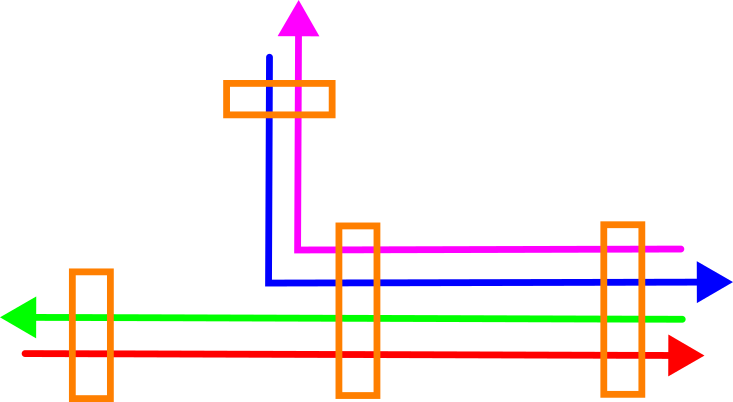
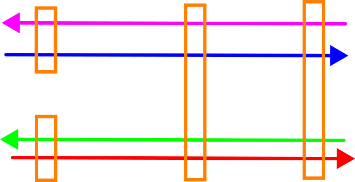
Below drawing shows a side view of this situation. The purple and blue driveline are close together, as are the green and red driveline – but there’s a systematic offset between the two pairs. This is not an uncommon occurrence, especially when matching drivelines from multiple sessions.
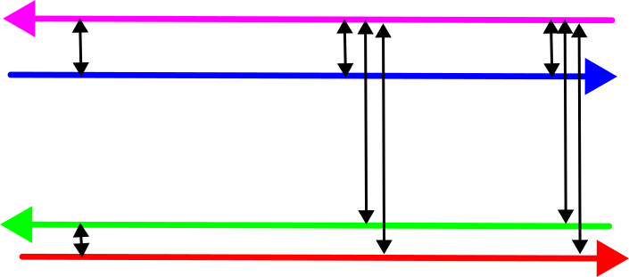
We can determine the offsets between the drivelines (black arrows) with a suitable method, then use them to generate corrections that bring the drivelines together. My HaiQuality Adjust software checks the resulting corrections against the a-priori stochastic model and modifies it where necessary to get proper weighting of the individual drivelines. This prevents drivelines of poor quality from disturbing the overal solution.
 Unfortunately, when each location is treated individually, branching drivelines can lead to deformations in the data. In our example case, the drivelines are “bent” and quickly diverge beyond the location where all of them are matched.
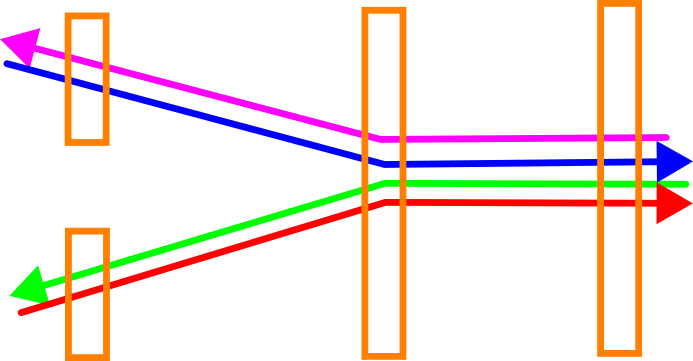
This can be remedied by introducing additional observations (orange arrows) that link the locations with each other:
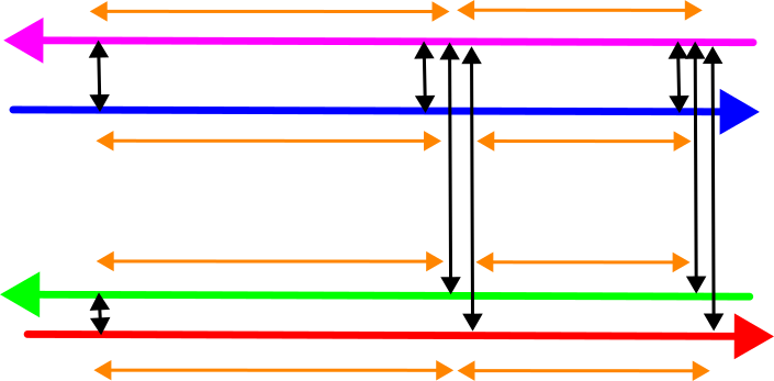
We thus obtain the following observations:
- The differences between the overlapping drivelines at each adjustment location. These are given a very high weight to ensure that the corrected data matches exactly.
- The links between the adjustment location. These have an observation value of 0, but a lower weight that should depend upon the accuracy of the trajectory segment.
Our unknowns are the corrections at each matching epoch, i.e. one for each adjustment location and driveline.
The result is a network that can be adjusted in a least-squares way. The functional model is very simple and linear, consisting only of -1 and 1 values in the design matrix – just like a levelling network. Without ground control points, the normal matrix is ill-conditioned, so the Moore-Penrose pseudo-inverse is used to compute the adjusted parameters. Iterative re-weighting can once again be used to tune the stochastic model. This doesn’t even require computing the residuals, as the computed corrections for the two epochs that make up a link can be used for that.
So much for the theory, but does it work in practice? Here’s an example of a rail project. The data acquisition was done under difficult conditions (low speed, relatively long baselines, high ionospheric activity, stopping under platform roofs with very poor GNSS reception) over three days, with almost 30 drivelines required for full project coverage. This resulted in relatively large corrections for some drivelines. The track layout is complex including a marshalling yard, leading to multiple locations where tracks and thus drivelines diverge and no longer overlap.
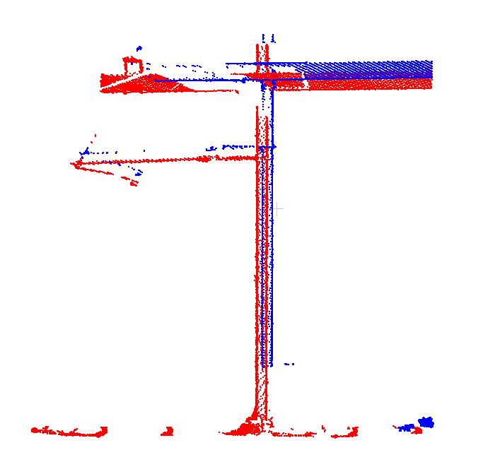
Let’s look at the “old” approach first, which treats each adjustment location in isolation. Here’s a plot of the point clouds of two drivelines after adjusting at a common location:
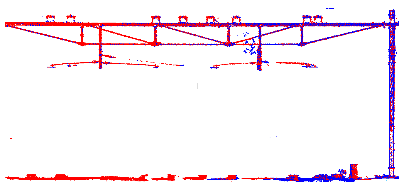
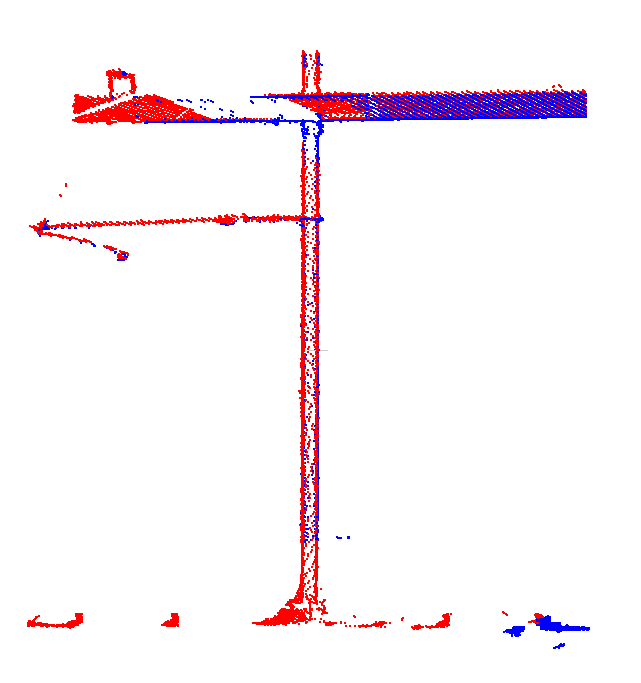
And here they are at a different location whey they have not been adjusted together, as there’s very little overlap. They have already diverged quite a bit:
 Here’s the first location resulting from the corrections computed with the new adjustment approach. Once again, both drivelines are nicely matched:
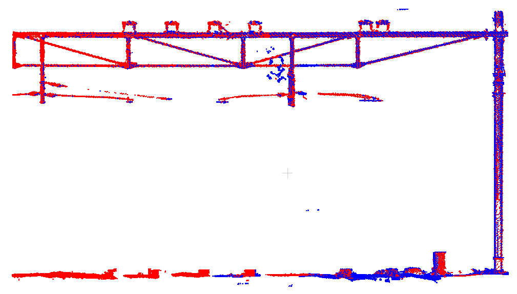 And here’s the second location. Despite not being part of a common adjustment location, i.e. with no direct links between them, the full network adjustment ensures that both drivelines still match nicely:
 The nice thing about this new approach is that it does not entail more work, as it still only needs the differences between overlapping tracks. Better quality for the same amount of work, what else can you wish for?